This tutorial is going to show you how to create a drop-down list in Excel.  I think it’s one of those features that everyone should know how to do – it saves time and is very useful 🙂

It uses a function called Data Validation, which basically means users can only input data which is valid, data which you have specified.

Part 1 shows how to create a basic list using data contained in the same worksheet.  Part 2 shows the data being contained in a different worksheet to the list.

Part 1

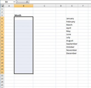
For example, we have a column with the heading Month, only months of the year can be input into this column so we need to set up a drop-down list specifying the months of the year, this way the user can only input what’s included in the list.

To set this up we first need to type the list, in this case the months of the year.  Then highlight the column or area where we want the drop-down list to appear…

Next, we go to the Data tab on the ribbon and select Data Validation…

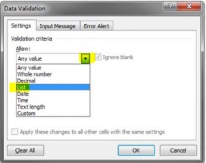
This will open a dialogue box where we enter the criteria for the data. Select List on the drop-down arrow where it says Allow…

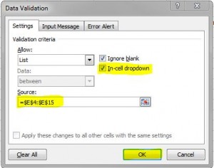
Another option then appears where we specify the range that contains the items (in this example it’s the list of the months in cells E4:E15).  Make sure In-cell drop-down is ticked and click OK…

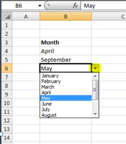
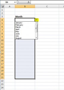
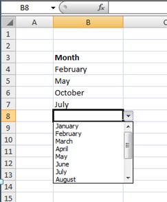
You’ll notice a little drop-down arrow has now appeared to the right of the first cell in the highlighted area. If we click on the arrow, the list of months should appear for us to select from…

And that’s how to create a drop-down list.  This example had the list of months in the same worksheet as the cell that contains the drop-down.

Part 2

If we want our list to be in a different worksheet then we would have to provide a name for the range that contains the list.

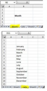
For example Sheet 1 is where we want the drop-down selection to be, and Sheet 2 (called Lists) is where the list is located.

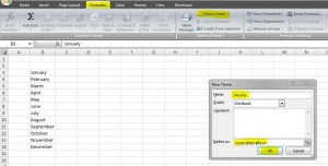
We want to name our range “Months”, so highlight the list of months, select Formulas tab on the ribbon and click Define Name.  Type in the name and you’ll notice the Refers to box already has the range in there (because we highlighted the months first), click OK.

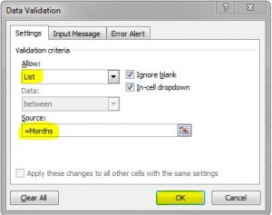
Go back into Sheet 1 and highlight the area where we want the drop-down to appear, select the Data tab in the ribbon and Data Validation. Choose Allow List (the same as in Part 1), type in =Months in the Source box, and click OK…

And the drop-down arrow will appear containing the months…

And that’s it!  There are other options for data validation i.e. text length, date, time etc, but the drop-down list is, in my opinion, one of the easiest and most useful to know .

I’ll cover the others in future tutorials 🙂