A client was amazed this week when he saw a cell “magically” change colour after I entered a certain value into it.  After briefly explaining how I’d done this, I thought I’d share this Excel feature for others who may not know how to use it 🙂

Conditional formatting is used when you want to change the appearance of a cell depending on certain conditions; for example, if you have a table showing sales, you may want to pick out the values over a certain amount, with conditional formatting you can set the cells to automatically be a different colour.

Below is a step by step guide on how to do it:-

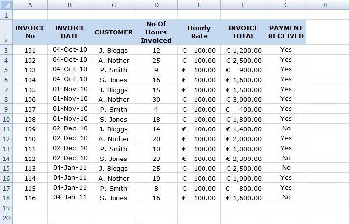
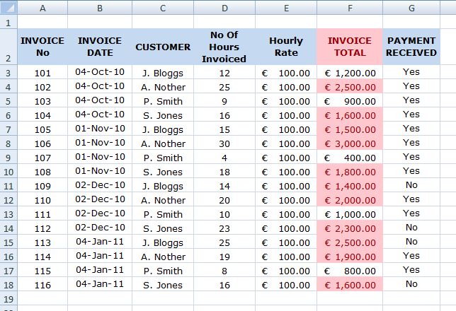
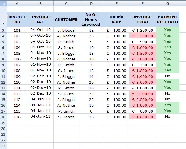
The following spreadsheet shows monthly invoicing amounts

(**NB This table does not reflect my hourly rate or my invoicing amounts – I wish they did!) 😉

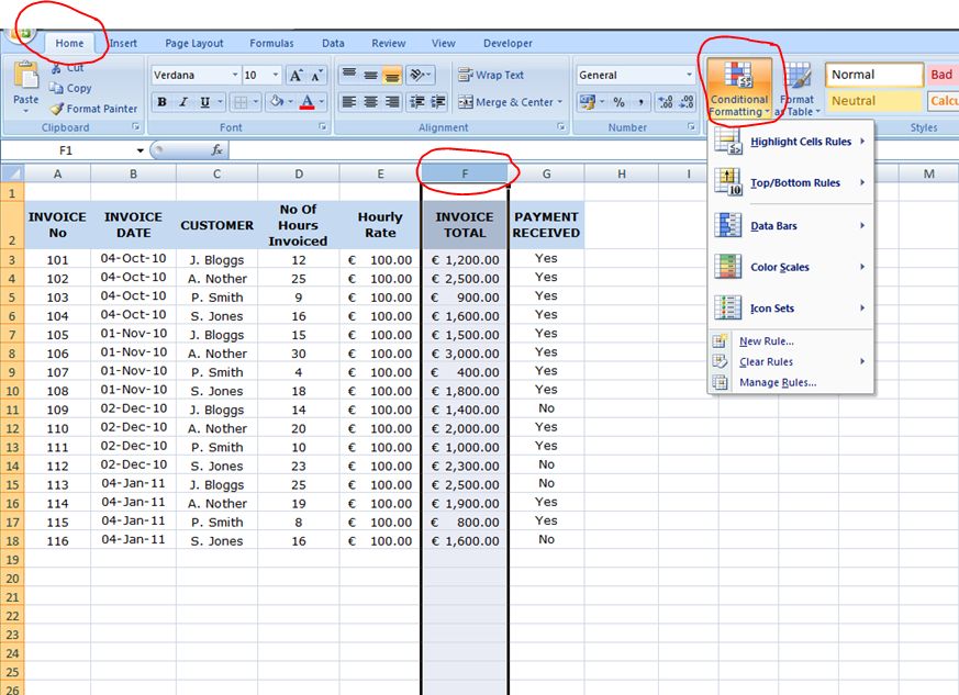
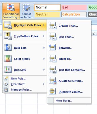
So, lets say we want to see all total invoiced amounts over €1200, firstly we need to highlight the Invoice Total column, then in the Home menu, select Conditional Formatting, this will drop down a menu where we can choose to highlight cell rules, top/bottom rules, data bars, colour scales, icon sets.

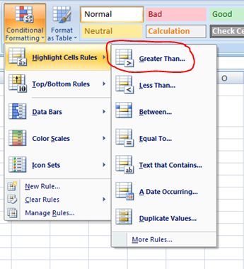
We need to click on Highlight Cells Rules and select Greater Than…as we want to set a condition to show cells with a greater value than €1200.

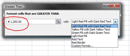
This will then open a dialogue box asking us to enter the value we wish the cell to be greater than (i.e. €1200), we then select the colour formatting we  want the cells to undertake.

Once we have chosen the colour and clicked okay, all of the cells over €1200 within the Invoice Total column will now be a different colour.  And, because the whole column was selected to begin with, it means any future amounts entered on this spreadsheet will automatically have the same formatting.

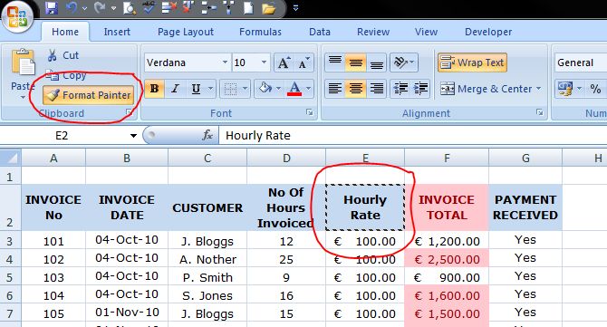
Another thing you may have noticed is that the Invoice Total column header also changed colour.  To change this back again a simple way of copying a format from one cell to another is Format Painter.  This icon is located in the Clipboard section of the Home menu.

To use this we first click on the cell whose format we want to copy – we’ll be copying the Hourly Rate header cell.  Then click the Format Painter icon and you’ll notice a flashing dotted line appear around the cell we selected.

Then, click on the cell we want to be pasted and the format changes immediately.

Other format conditions we can choose are Less Than, Between, Equal To – these work in the same way as the Greater Than rule.  We can also choose cells which has Text that Contains, Date Occurring (i.e. yesterday, last month etc), or Duplicate Values.

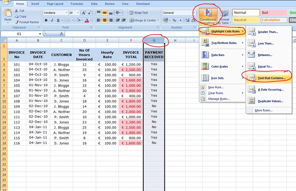
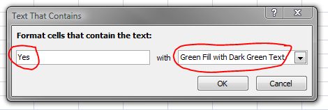
Lets choose Text that Contains as another example.  All invoices where payment has been received we want the Yes to be shaded in green so, we highlight the Payment Received column, go to Conditional Formatting, select Highlight Cells Rules and Text that Contains…

Type in the text that the cell must contain in order to be formatted (i.e. Yes) and choose the colour that we want the cell to change to (i.e. green)

All the cells within that column that contain the text Yes will now change to green.  Again, because the whole column was selected, it means future entries will automatically be formatted the same way.  You’ll notice the column header didn’t change this time, this is because it didn’t contain the relevant text (i.e. Yes)

I hope this has been helpful to anyone who doesn’t know much about formatting cells – of course, there are many more formatting rules and options which I haven’t covered yet.  This was just a basic example to get you started! 🙂