A client was amazed this week when he saw a cell “magically” change colour after I entered a certain value into it.  After briefly explaining how I’d done this, I thought I’d share this Excel feature for others who may not know how to use it 🙂

Conditional formatting is used when you want to change the appearance of a cell depending on certain conditions; for example, if you have a table showing sales, you may want to pick out the values over a certain amount, with conditional formatting you can set the cells to automatically be a different colour, font and style.

Below is a step by step guide on how to do it:-

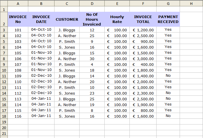
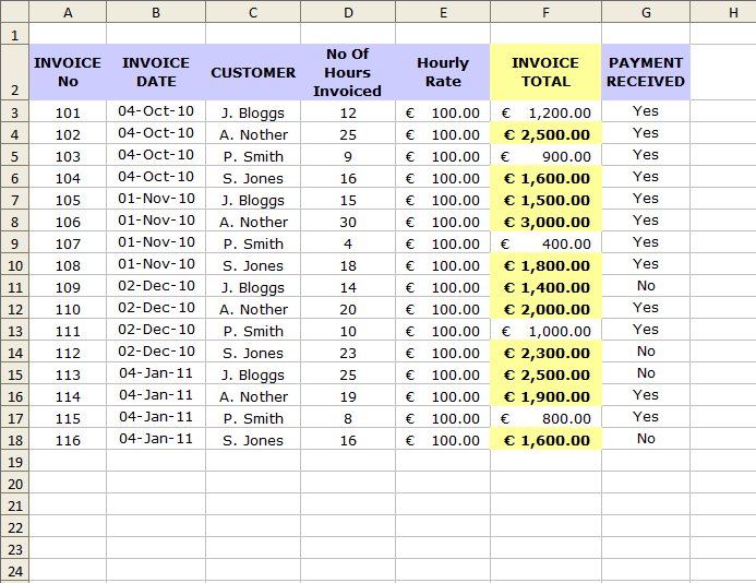
The following spreadsheet shows monthly invoicing amounts:-

(**NB This table does not reflect my hourly rate or my invoicing amounts – I wish they did!) 😉

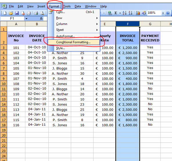
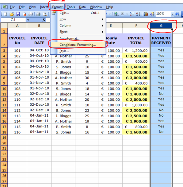
So, lets say we want to see all total invoiced amounts over €1200, firstly we need to highlight the Invoice Total column, then we click on Format in the toolbar and select Conditional Formatting.

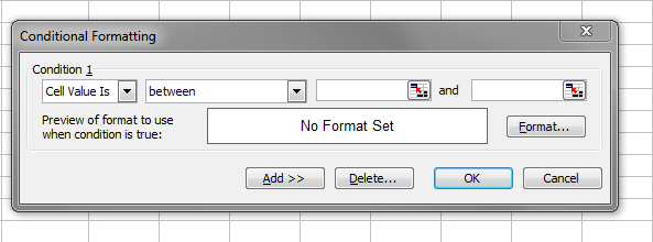
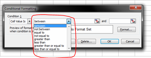
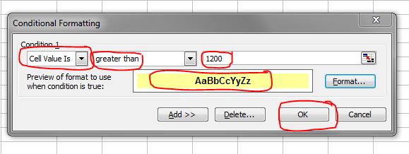
This will open a dialogue box where we can choose the conditions we want to set.

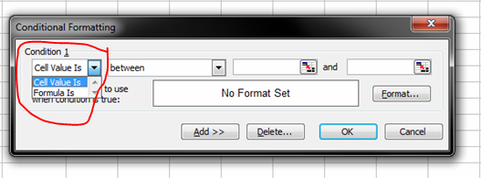
Clicking on the arrows to the right of the text will drop down menus offering different options.  The first one gives us the option of choosing either the cell value is or the formula is.  This means we can either set conditions for the values contained in the cells or specific formulas within the highlighted range.

The next drop down arrow gives the selection of the criteria we want the cell to have i.e. greater than, less than, between…..

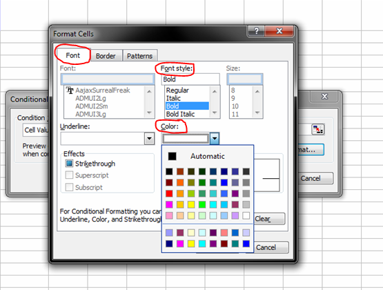
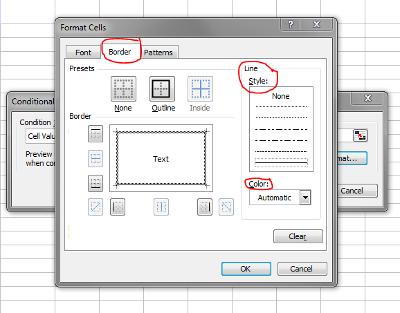
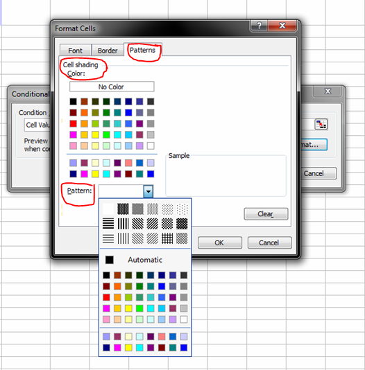
The final selection is the formatting – this takes us to another dialogue box where we can format the font, border and pattern.

So, we want to select Cell Value is greater than 1200 and we’ll make the cells turn yellow and change the font to bold.

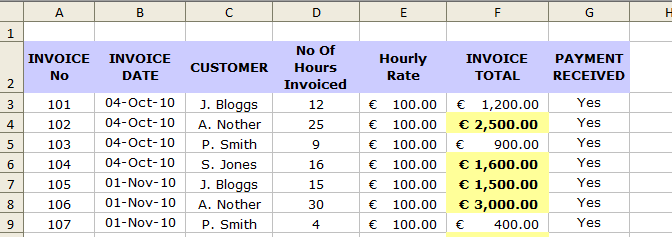
Once we have chosen the colour and clicked okay, all of the cells over €1200 within the Invoice Total column will now be a different colour.  And, because the whole column was selected to begin with, it means any future amounts entered on this spreadsheet will automatically have the same formatting.

Another thing you may have noticed is that the Invoice Total column header also changed colour.  To change this back again a simple way of copying a format from one cell to another is Format Painter.  This icon is located on the Toolbar at the top of the screen.

If ever you’re unsure of what an icon does, just hover over it and it will tell you 🙂

To use this we first click on the cell whose format we want to copy – we’ll be copying the Hourly Rate header cell.  Then click the Format Painter icon and you’ll notice a flashing dotted line appear around the cell we selected.  Then, click on the cell we want to be pasted and the format changes immediately.

Other format conditions we can choose are Less Than, Between, – these work in the same way as the Greater Than rule.  We can also choose cells which contain certain text by using the equal to rule.

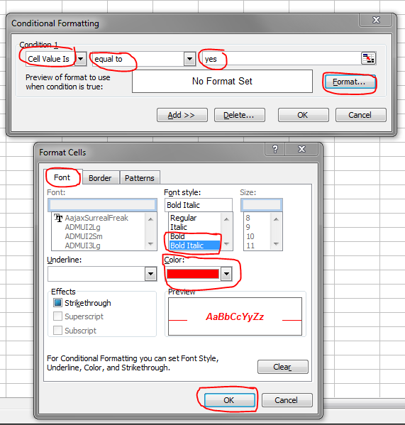
Lets choose Equal to as another example.  All invoices where payment has been received we want the Yes to be in red, bold italic text, so we highlight the Payment Received column, go to Format on the Toolbar, and select Conditional Formatting.

We select Cell Value is and equal to, then we type in the text that the cell must contain in order to be formatted (i.e. Yes) and click on Format.  The next dialogue box opens where we choose the font style and colour (i.e. Bold Italic & red)

All the cells within that column that contain the text Yes will now change to red.  Again, because the whole column was selected, it means future entries will automatically be formatted the same way.  You’ll notice the column header didn’t change this time, this is because it didn’t contain the relevant text (i.e. Yes).

I hope this has been helpful to anyone who doesn’t know much about formatting cells – of course, there are many more formatting rules and options which I haven’t covered yet.  This was just a basic example to get you started! 🙂