For years if I had a list in Excel that was all in Capitals (or lowercase) and I wanted to change the text case, I either used to retype the whole thing again or copy & paste it into Word, highlight it all and change to upper/lower case that way.

I then found out a way in Excel that saves so much time…… use formulas to change the text case 🙂

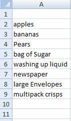
If, for example, Column A contained text which was a mixture of upper and lowercase letters – it might look a bit messy, it may only be your shopping list, but it still doesn’t look right!

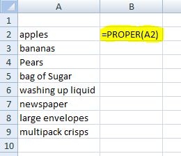
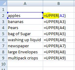
So you want to tidy it up a bit and have all words begin with a capital letter.  Go into the next blank cell and use the formula “proper” to change it:-

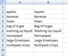
Then use the autofill handle (bottom right corner of the cell) and drag the formula down to the end of your list (or copy & paste the formula down, whichever you prefer).  This then duplicates your list in proper text i.e. capital letter at the start of every word.

Of course, now when you delete the text in column A, everything in column B disappears! This is because it still contains a formula linking to the text in column A.  To rectify this, you need to paste special the cells.

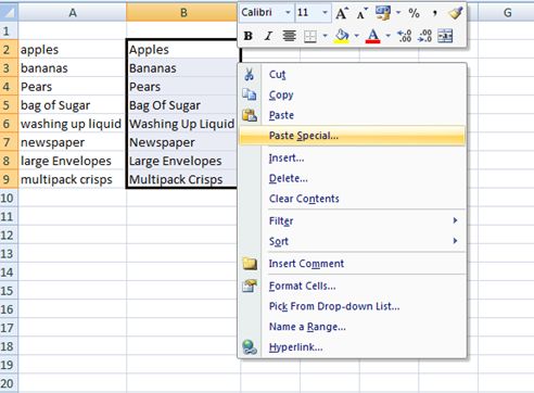
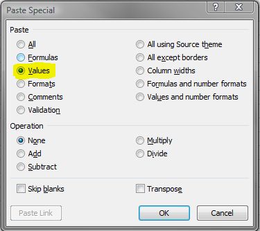
Highlight the text in column B (all cells which contain a formula), click Copy (or press Ctrl+C), then right click the mouse and select Paste Special…

This will open another menu where you can choose how you want to paste the cells.  You want to get rid of the formulas and just keep the actual value/text of the cell, so click on Values and press OK.

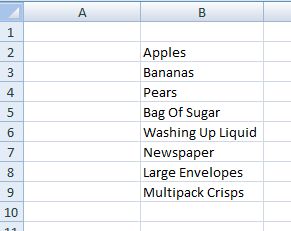
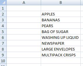
You’ll then notice that column B, which had the formula in, now contains the correct text – and you can now delete everything in column A

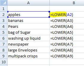
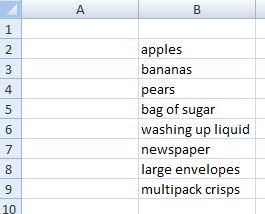
The same method applies if you want the text all in capitals, or all in lower case – the only change is the formula.

For CAPITALS, use:-

Then copy and paste special values as before.

For lowercase, use:-

Again copy & paste special values as before.

And that’s it – hopefully it will save you time, instead of having to type things out again (like I used to ;))