When working in a spreadsheet there may be a time when you don’t necessarily want to see all of the sheets. For example, one of the sheets may contain the lists that are being used for the drop down data, which you don’t need to see. Hiding the sheet will have no effect on any formulas or references and data contained in that sheet can still be used in other worksheets. This short video will show you how to do this in version 2007 / 2010. A step by step guide is below the video too 🙂
In my example I have 3 sheets called Sales, Purchases and Lists. I want to hide the Lists worksheet.
Method 1 – the ribbon way
Make sure you’re in the worksheet you want to hide (if you’re not then just click on the tab of the worksheet you want to hide)…
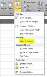
Click on the Home tab in the ribbon, and go to the Cells section…
Click on the Format drop down arrow, and choose Hide & Unhide in the Visibility section…
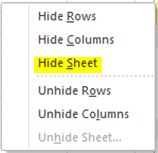
Then select Hide Sheet to hide the current worksheet…
The worksheet will now be hidden…
If you want to hide more than 1 worksheet, click on the first worksheet you want to hide, then hold down Ctrl and click on the tabs of the other worksheets you want to hide and follow the above steps.
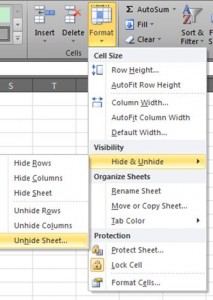
To unhide any hidden worksheets go to Cells section on the Home tab of the ribbon, click on Format, choose Hide & Unhide and select Unhide Sheet…
This will open up a dialogue box listing all worksheets that are currently hidden, just select the sheet that you want to unhide and click OK…
The worksheet has now reappeared.
Method 2 – the mouse way
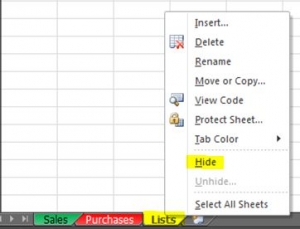
As above, make sure you’re currently in the worksheet that you want to hide, then just right click on the Sheet name – in this example it’s Lists, and select Hide…
And that’s it, Lists becomes hidden! To unhide, again just right click the mouse on any sheet name, and choose Unhide. A dialogue box listing all worksheets that are currently hidden will open, just select the sheet that you want to unhide and click OK. Simple 🙂


