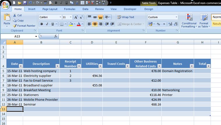
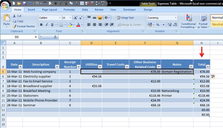
To pick up from the last tutorial, below is the expenses table – you’ll notice I’ve filled in a few more rows.

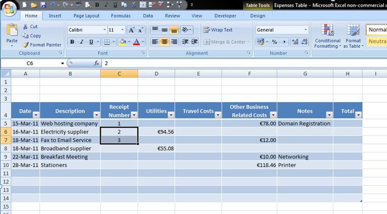
I’ve deliberately not filled in the Receipt Number column as we’ll use the Autofill feature to save time.  Highlight the last 2 numbers entered in the receipt number column (i.e. 2 and 3).

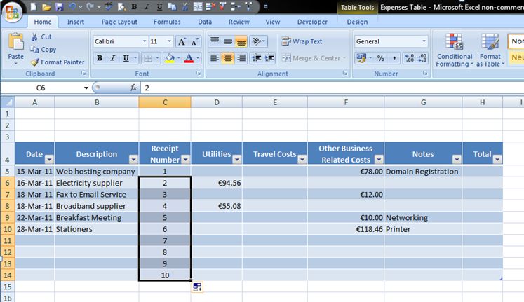
Hover the cursor over the bottom right corner of the highlighted cells until it changes to a “+” sign.  Double click and it will automatically fill the rest of the cells in that column in the table, or click and drag down and it will automatically fill in the empty cells beneath following the same sequence.

The same procedure applies for any sequence of numbers i.e. 2, 4, 6, 8 etc, and for days / months.

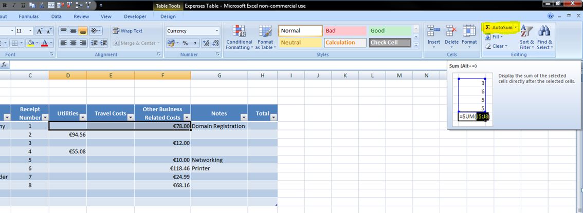
We now want to add together the figures in the total column.  Highlight the cells in the first row that you want to total, in this case everything from Utilities (column D) to Other Bus Rel Costs (column F).  Click on the Autosum button within the Editing section on the ribbon, in the top right corner.

The total appears in the next cell available and automatically copies it down to the end of the column.

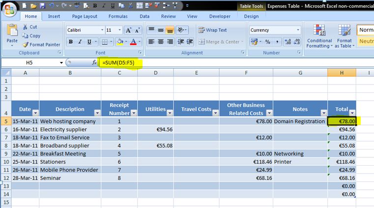
If you click on a cell within the Total column, you can see the formula in the bar at the top, so it’s totalling the cells in columns D to F.

You can delete the formula from any cells that you don’t want it in (i.e. row 13 & 14 in above picture).

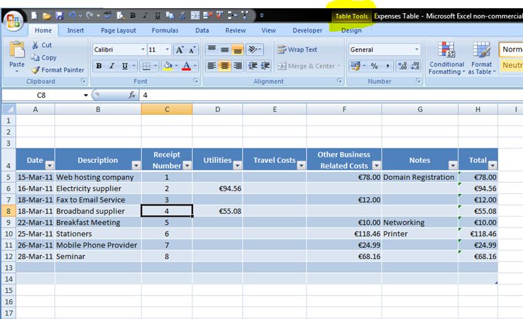
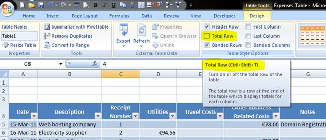
So, we now have totals for each row, but we also want a grand total for the whole table.  Click once anywhere within the table and you’ll notice Table Tools appears at the top of the toolbar.

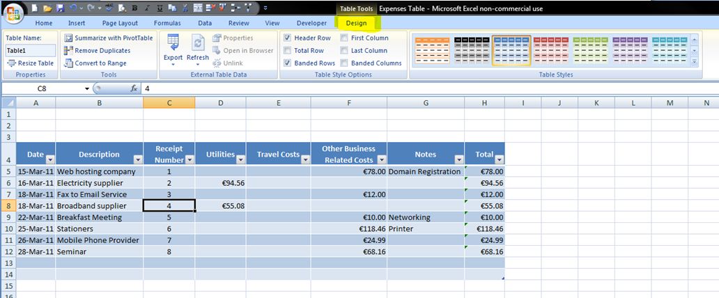
Click on Design immediately below that and different options appear for formatting the design of the table.

In Table Style Options, tick the box called Total Row – hover over it and it will also describe what it does and give you the shortcut (Ctrl + Shift + T).

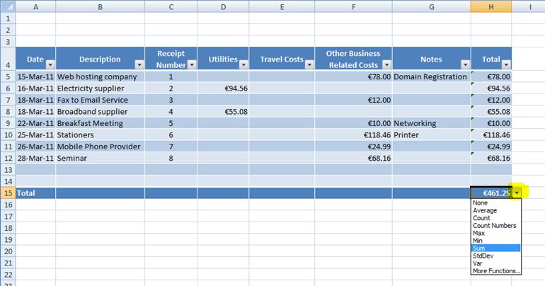
Once ticked, a total row will appear at the bottom of the table.  If you click on the cell containing the grand total, a drop down arrow appears – click on it and it gives you other options besides sum.

This is handy if, for example, we want to know the average of the totals, or the number of entries made in the table (count).

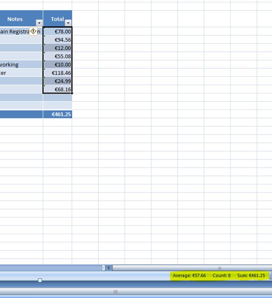
Another way of checking this is to highlight the total cells (excluding the grand total), and look at the bottom of the screen.  Excel 2007 automatically shows the average, count and sum of any cells you highlight (a handy feature :)).

So, there we have a basic table to show expenses and totals – my next tutorial will be on how to format it ready to print 🙂